Linear regression using some of the popular software

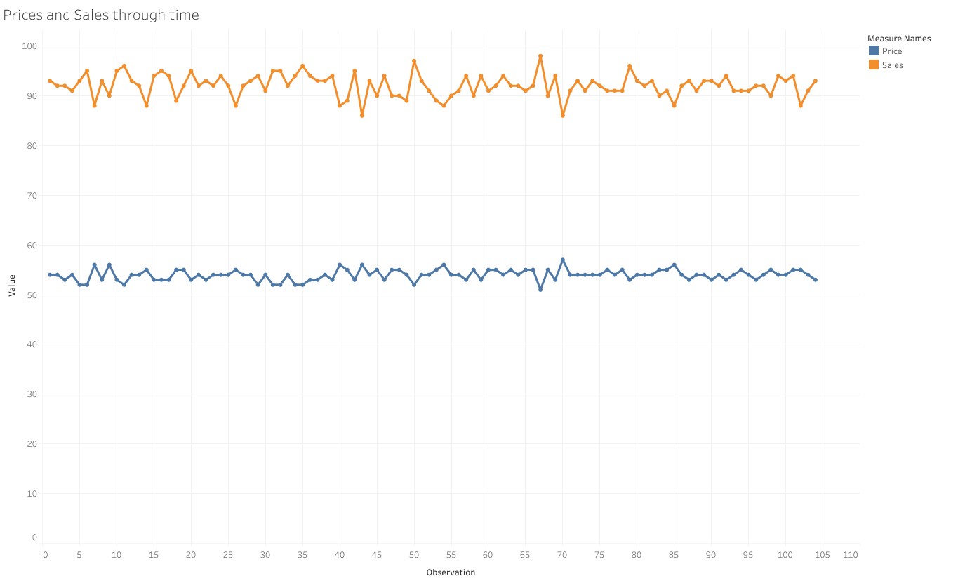
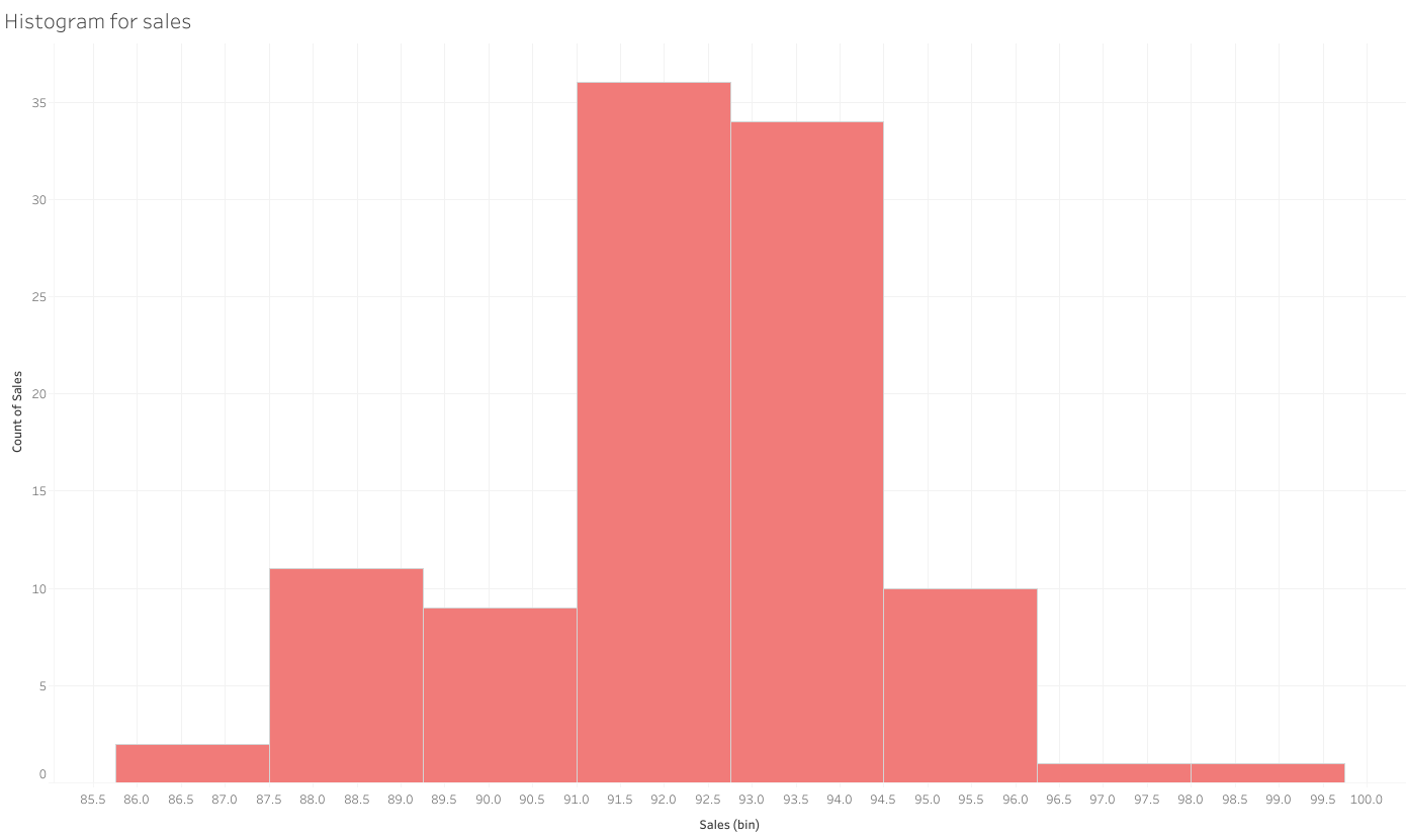
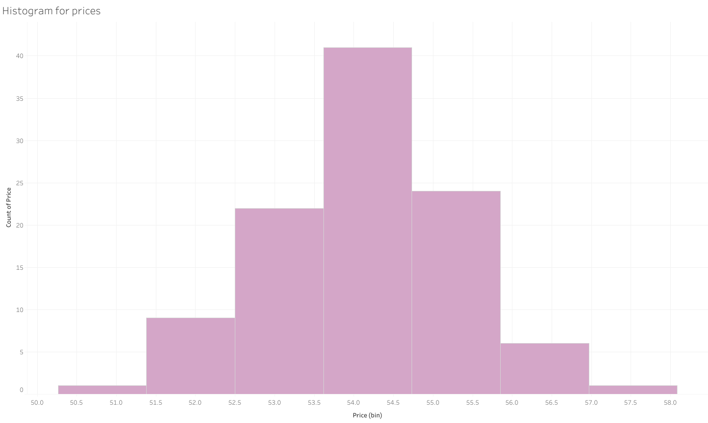
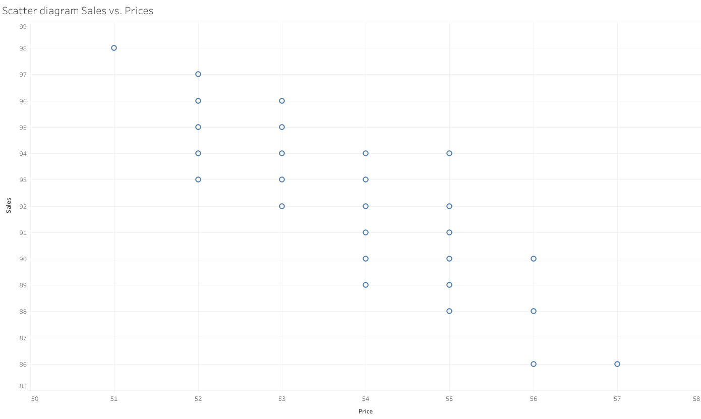
I use the data (in the form of ‘Dataset1.xls’ or ‘Dataset1.txt’ both consist the same data ) from an online course “Econometrics: Methods and Applications” by Erasmus University Rotterdam. The data includes two variables “Price” and “Sales”, while the former is independent variable and the latter is dependent variable.

Let’s get to it!

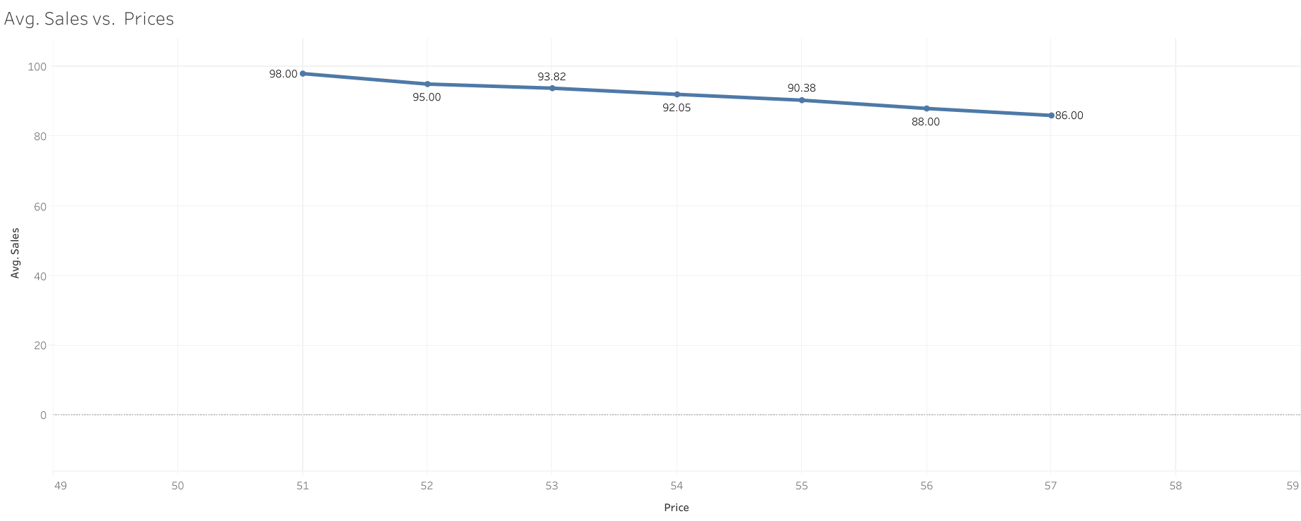
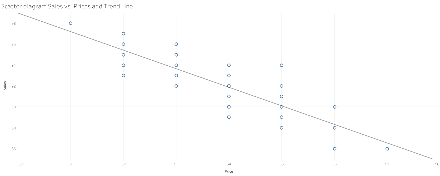
First some data viz using #Tableau :

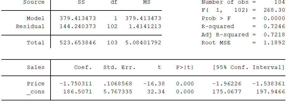
Regression using #Stata:

Input:

cd "C:\Users\Yours"
import excel Dataset1.xls, firstrow
reg Sales Price 

Output:

Regression using #R:

input:

setwd("C:/Users/Yours")
library("xlsx")
Sys.setlocale(category = "LC_ALL", locale = "english")
week1 <- as.data.frame(read.xlsx("Dataset1.xls", sheetName = "Dataset 1"))  
regression <- lm(Sales~Price, data = week1)
summary(regression)

output:

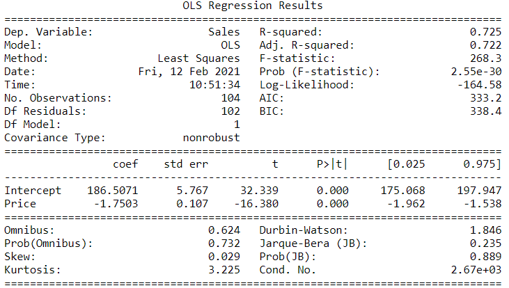
Call:
lm(formula = Sales ~ Price, data = week1)

Residuals:
    Min      1Q  Median      3Q     Max 
-2.9904 -0.7407  0.0096  1.0096  3.7599 

Coefficients:
            Estimate Std. Error t value Pr(>|t|)    
(Intercept) 186.5071     5.7673   32.34   <2e-16 ***
Price        -1.7503     0.1069  -16.38   <2e-16 ***
---
Signif. codes:  0 ‘***’ 0.001 ‘**’ 0.01 ‘*’ 0.05 ‘.’ 0.1 ‘ ’ 1

Residual standard error: 1.189 on 102 degrees of freedom
Multiple R-squared:  0.7246,	Adjusted R-squared:  0.7218 
F-statistic: 268.3 on 1 and 102 DF,  p-value: < 2.2e-16

Regression using #Python:

input:

import os
import pandas as pd 
import statsmodels.formula.api as sm
os.chdir('c:\\Users\\Yours')

week1 = pd.read_excel('Dataset1.xls')
regression = sm.ols(formula="Sales ~ Price", data=week1).fit()
print(regression.summary())

output:

Regression using #Octave:

Input:

cd "C:\\Users\\Yours"
week1 = dlmread("Dataset1.txt");
Price = week1(:, 2); 
Sales = week1(:, 3);
Price = Price(2:end); 
Sales = Sales(2:end);
m = length(Price)
PriceWithBias = [ones(m,1), Price(:,1)];
parameters = (pinv(PriceWithBias'*PriceWithBias))*PriceWithBias'*Sales 
parameters

Output:

  parameters =

   186.5071
    -1.7503

Coming up next Regression using #Julia!!!

See you in another post!